Intro to Numpy and Simple Plotting

In this lesson you will be introduced to Numpy, and some simple plotting using pylab. A simple script will be introduced that opens a spreadsheet of data, computes some simple statistics, creates some simple plots.

Numpy = Numerical + Python

Numpy is the main building block for doing scientific computing with python. A wealth of information can be found here:

http://numpy.scipy.org

Numpy for Matlab users

As an object-oriented language, python may seem very different than matlab, and in many ways it is. However, for people with a Matlab background it can be fairly easy to switch to python using Numpy. These pages can be very useful to understand:

• which numpy function maps to a given matlab function
• difference between numpy array and numpy matrix
• how to index arrays, and fancy indexing

http://mathesaurus.sourceforge.net/matlab-numpy.html

http://www.scipy.org/NumPy_for_Matlab_Users

Script Deconstruction : numpy_example.py

numpy_example.py

In this example, I will open a file (this one uses colon : as a delimiter), and I will read in different fields so I can analyze and viualize the data.

import

import numpy as np

This is the main tool used in the rest of this script.

Parse the Header

I know my data file has a header row as its first row of data. So I plan to read this in and use this to help load in the rest of my data.

The beginning of the first row looks like this:

"BAC#":"Gender":"Handedness":"Years Ed":  ...

As you can see

• Fields are separated by colon :
• There are extra quotes ” in the fields

So I will

• read in the first line
• strip unnecessary quotes
• split on the colon to create a list
• cast result to a numpy array

code:

infile = 'Cindee_11_9_10_v2.csv'
hdrstr = open(infile).readline()
hdrs = hdrstr.replace('"','').split(':')
hdrs = np.array(hdrs)

So Now I want to find the indicies of a field, lets say all the fields that have ‘BAC’ in them:

bac_ind = [np.where(hdrs==x) for x in hdrs if 'BAC' in x]
bac_ind = [x[0][0] for x in bac_ind] #simplify
bac_hdr_str = hdrs[bac_ind]

np.where returns indicies where a logical test on an array returns true

so this lets me find the indicies of the fields that have the term “BAC” in them....

Using loadtxt

Now that I have figured out what fields I want, Ill use np.loadtxt to load them into an array so I can work with the data:

np.loadtxt(fname, dtype=<type 'float'>, delimiter=None, skiprows=0, usecols=None)

np.loadtxt

• fname = filename of text file to open
• dtype = base datatype to cast data to
• delimiter = character used to specify boundry between fields
• skiprows = number of leading rows to skip (in case you need to skip headers)
• usecols = tuple indicating the specific columns of data you wish to extract

example:

mydata = (0,1,3,6,10,36)
dat = np.loadtxt(infile, delimiter=':',
                 dtype=np.str, usecols=mydata,
                 skiprows = 1)

array([['"BAC001"', '"F"', '18', '63', '30', '13'],
      ['"BAC002"', '"M"', '18', '70', '30', '7'],
      ['"BAC003"', '"F"', '14', '61', '30', '12'], ...

Im skipping the first row since I already have dealt with getting my headers. And Im casting the data to a dtype of string np.str because the columns I am grabbing have mixed types, I will re-cast them to the correct types later. I could also load different types separately to avoid this issue.

Grab MMSE out of the dat array, replace missing fields, and cast to float:

empty = np.where(dat[:,keys['mmse']]=='')
dat[empty,keys['mmse']] = np.nan
mmse = dat[:,keys['mmse']].astype(np.float)

array([ 30.,  30.,  30.,  28.,  30.,  29.,  28.,  30.,  28.,  29.,  29.,
        28.,  30.,  30.,  NaN,  29.,  29.,  30.,  30.,  30.,  30.,  29.,

Simple Statistics

I may want to calculate a simple mean. But this will be an issue as I have NAN in the array. however, it is simple to mask the array:

mmse_mean = mmse[mmse>0].mean()
28.991735537190081
mmse[mmse>0].std()

To make this more interesting...... I now get arrays of data for CVLT and age. For each of these, there may be different regions where subjects have missing fields. So if I want to compare two variables, I need to find the places where they overlap:

overlap2 = np.logical_and(mmse>0, cvlt>0)

I can now use some other numpy toos to see how two measures relate to each other.

polyfit:

p = np.polyfit(mmse[overlap2], cvlt[overlap2],1)
array([  0.87076373, -13.59299814])
x = [mmse[overlap2].min(), mmse[overlap2].max()]
y = np.polyval(p, x)

least squares:

m = np.ones((mmse[overlap2].shape[0],2))
m[:,0] = mmse[overlap2]
results = np.linalg.lstsq(m, cvlt[overlap2])
print results[0]
array([  0.87076373, -13.59299814])

Simple Plotting

In simple situations like this I use the -pylab directive of Ipython if I want to generate some simple plots:

ipython -pylab

It requires matplotlib to be installed, but is a powerful tool. There is a wonderful set of example plots to be found here:

http://matplotlib.sourceforge.net/gallery.html

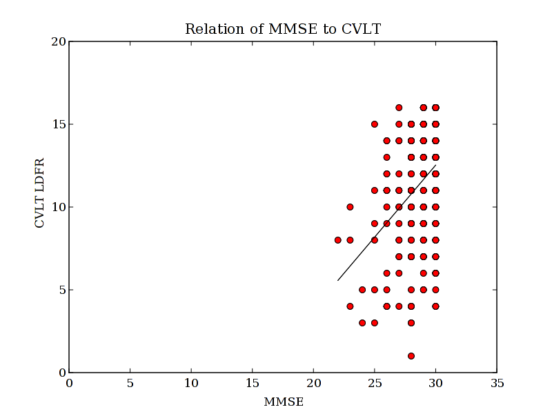
So if we want to see our mmse, and cvlt data:

plot(mmse, cvlt, 'ro')
plot(x,y, 'k-')
axis([0,35,0,20])
title('Relation of MMSE to CVLT')
xlabel('MMSE')
ylabel('CVLT LDFR')

Homework

1. Open a text file of (your own) data
2. Parse the header
3. Open the data and grab a subset of fields
4. generate a simple statistic and create a simple plot
5. save a png image

Email me if you get stuck, you have a few weeks